Norkyst model documentation#

The scientific basis and technical configuration of Norkyst v.3 are described in detail in the following peer-reviewed publication:

Christensen, K. H., Albretsen, J., Asplin, L., Frøysa, H. G., Gusdal, Y., Iversen, S. C., Jensen, M. F., Johnsen, I. A., Kristensen, N. M., Sævik, P. N., Sandvik, A. D., Simonsen, M., Skarðhamar, J., Sperrevik, A. K., and Trodahl, M.: “Norkyst” version 3: the coastal ocean forecasting system for Norway, Geosci. Model Dev., 19, 2785–2798, https://doi.org/10.5194/gmd-19-2785-2026, 2026.

All figures below are reproduced from Christensen et al. (2026) under the Creative Commons Attribution 4.0 License.

Model domain and grid#

Norkyst v.3 covers the full length of the Norwegian coast, from the Skagerrak in the south to the Barents Sea in the north. The model is formulated on a curvilinear rotated polar stereographic grid with approximately 800 m horizontal resolution, comprising 2747 × 1148 grid points. The maximum model depth is 3257 m, and roughly 42 % of the grid cells are land.

The bathymetry is derived from a combination of the EMODnet Digital Bathymetry dataset and high-resolution data from the Norwegian Mapping Authority. The depth matrix is smoothed using a Laplacian filter, and a minimum depth of 10 m is applied to maintain numerical stability while preserving realistic near-shore hydrodynamics.

The extended domain compared with earlier versions of Norkyst was designed to avoid cutting across the most eddy-active regions along the shelf break, and to capture the energetic exchange between coastal and open-ocean waters more faithfully. Where the horizontal resolution is insufficient to resolve narrow sounds or passages, these have been selectively opened or closed to achieve as realistic an overall circulation pattern as possible.

The vertical discretisation uses 40 terrain-following sigma layers, with enhanced resolution near the surface to support operational services that depend on near-surface currents (e.g. search-and-rescue, oil spill response, salmon lice dispersal). Typical vertical resolution near the surface ranges from about 0.1 m at 10 m water depth to approximately 1.0 m at 1000 m depth.

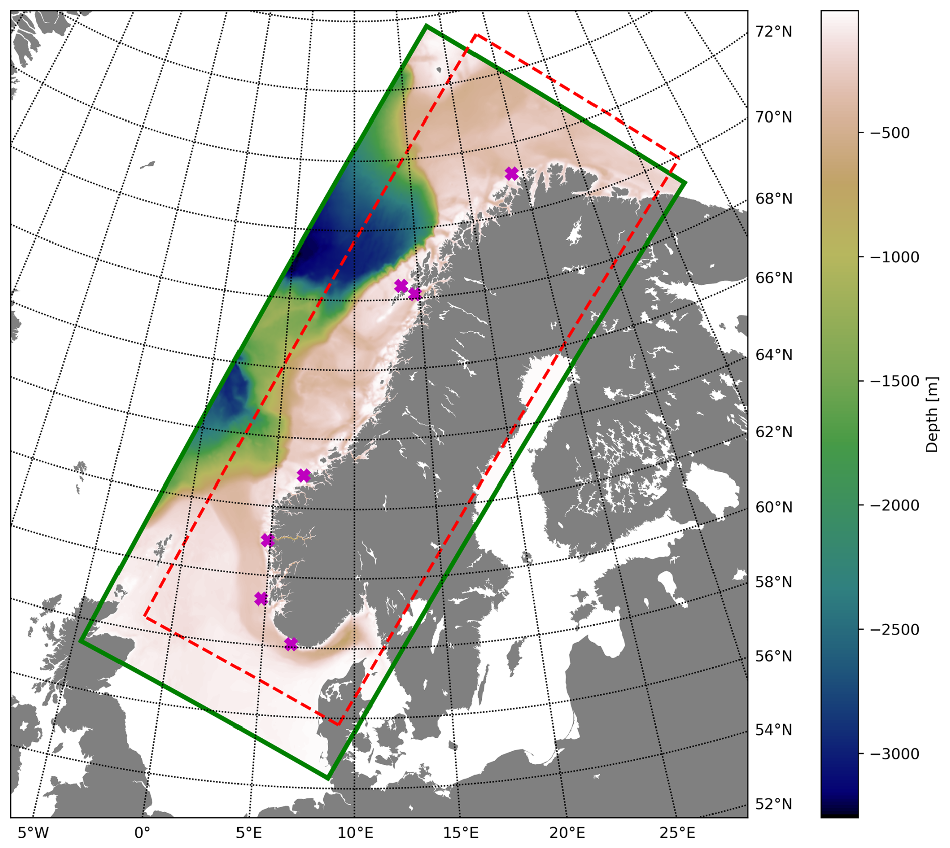
**Figure 1** — The Norkyst v.3 model domain and bathymetry (green solid line). The outline of the previous version of Norkyst is also shown (red dashed line). The domain extends from the North Sea in the south to the Barents Sea in the north. A pronounced shelf break separates the Norwegian coastal ocean from the Norwegian Sea to the west. Magenta crosses mark the positions of the IMR fixed coastal hydrographic stations used for model validation. *(Christensen et al., 2026, Fig. 1)*#

Dynamical core#

Norkyst is built on the Rutgers version of ROMS (Regional Ocean Modeling System; Shchepetkin and McWilliams, 2005; Haidvogel et al., 2008). ROMS solves the hydrostatic primitive equations on a staggered C-grid using a split-explicit time stepping scheme that separates the fast barotropic (surface gravity wave) mode from the slow baroclinic (density-driven) mode.

The primary prognostic variables are:

Depth-dependent horizontal velocities (u, v) and the tracer fields salinity (S) and potential temperature (T), associated with the slow baroclinic mode.
Depth-averaged horizontal velocities and the sea surface elevation (ζ), associated with the fast barotropic mode.

Time stepping: A baroclinic time step of 40 s and a barotropic time step of 2 s are used. The main stability challenge arises from large vertical velocities at strong convergence zones (e.g. the Kattegat–Skagerrak front), rather than from the horizontal resolution itself. The minimum model depth of 10 m is chosen partly to mitigate violations of the CFL criterion in the vertical tracer equations.
Advection schemes: Horizontal advection of momentum and temperature uses the default third-order upwind scheme. In the vertical, fourth-order centred schemes are applied. For salinity, the HSIMT (High-order Spatial Interpolation at the Middle Temporal level) scheme (Wu and Zhu, 2010) is used in both the horizontal and vertical directions, providing improved monotonicity near sharp fronts. No explicit lateral eddy viscosity is applied in the model interior, but a lateral diffusivity of 10 m² s⁻¹ is used for tracers.
Turbulence closure: Vertical turbulent viscosity and diffusivity are computed using the Generic Length Scale (GLS) scheme (Umlauf and Burchard, 2003) as implemented in ROMS (Warner et al., 2005). The GLS approach solves prognostic equations for turbulent kinetic energy (k) and a generic length scale (ψ), and uses stability functions from Canuto et al. (2001) (the CANUTO_A option) to relate eddy coefficients to the gradient Richardson number.
Sea ice treatment: Sea ice formation is infrequent along most of the Norwegian coast. Rather than coupling to a sea ice model, Norkyst v.3 activates a built-in ROMS parameterisation (LIMIT_STFLX_COOLING) that suppresses further cooling of the surface layer once the water reaches its freezing point, emulating the insulating effect of an ice cover. A dedicated coupled ocean–sea ice system for the Barents Sea and Svalbard region is maintained separately (Röhrs et al., 2023).

Forcing#

Atmospheric forcing#

For operational forecast production, Norkyst uses atmospheric fields from the AROME-MetCoOp numerical weather prediction system (Müller et al., 2017), operated jointly by the Nordic meteorological services. AROME-MetCoOp has a horizontal resolution of 2.5 km and provides output at 1 h intervals. For the small portions of the Norkyst domain that lie outside the AROME-MetCoOp grid (south-western and north-western corners), fields from the ECMWF medium-range HRES forecast (IFS) are used to fill the gaps.

For the hindcast archive, atmospheric forcing varies by period:

2012–2016: 3 km WRF simulations (Asplin et al., 2020) for wind, humidity and temperature; downwelling radiation from NORA3 (Haakenstad et al., 2021, 2022).
2017–2020: AROME-MetCoOp for wind, humidity and temperature; NORA3 for downwelling radiation. A warm bias of up to 0.7–0.8 °C in the surface layer during summer has been identified for this period, linked to an overestimation of solar radiation in NORA3.
2021–present: AROME-MetCoOp for all variables.

Surface heat and momentum fluxes are computed using the COARE 3.0 bulk flux scheme built into ROMS. Shortwave and downwelling longwave radiation are prescribed directly from the NWP system; the COARE algorithm then computes the net longwave flux. Atmospheric pressure is included in the forcing so that storm surges and tide–surge interactions are represented. Internal shortwave heating uses a Jerlov water type III profile, consistent with average Sentinel-3/OLCI observations over the model domain.

River discharge#

All rivers are represented with a prescribed volume flux, temperature, and a Froude-number-dependent vertical outflow profile that confines smaller river outflows closer to the surface. Daily discharge data for Norwegian rivers come from the Norwegian Water Resources and Energy Directorate (NVE), distributing total runoff for 69 coastal regions to 1760 river outlets (247 in the current operational setup) weighted by upstream catchment area. Runoff from Swedish, Danish and Scottish rivers is obtained from the E-HYPE European hydrological model (Donnelly et al., 2016).

Salinity is set to 1 PSU for all river inputs. River temperature follows a Gaussian seasonal cycle, with a maximum on 5 August, a standard deviation of 50 days, and a minimum of 2 °C. The peak temperature is parameterised as a function of latitude and fjord index to account for cold glacier meltwater in deep inner fjords:

\[T_{\mathrm{max}} = (-0.7 \times \mathrm{Latitude} + 59)\,(1 - 0.4 \times I_{\mathrm{fjord}})\]

where I_fjord is a fractional index between 0 (open coast) and 1 (innermost fjord).

Lateral boundary conditions#

Norkyst requires open boundary conditions on all four sides of the domain. The main inflow pathways are Atlantic water through the western boundary, North Sea water through the southern boundary, and Baltic Sea water through the eastern boundary. The eastern boundary runs through the central Kattegat, chosen to keep the fluctuating Kattegat–Skagerrak front fully within the model domain.

Boundary conditions are primarily sourced from the Copernicus Marine Service Arctic Monitoring and Forecasting Centre (ARC MFC), with the southern portion of the eastern boundary supplied by the Baltic Monitoring and Forecasting Centre (BAL MFC). Implementation follows the radiation/nudging approach of Marchesiello et al. (2001), using daily mean fields from the coarse-resolution parent models. Tidal forcing uses the TPXO9 tidal constituent database (Egbert and Erofeeva, 2002). A 40-grid-point relaxation zone with gradually increasing lateral diffusivities (10 to 50 m² s⁻¹) is applied toward the open boundaries. Nudging time scales are 15 d for outgoing signals and 0.5 d for incoming signals. The inverse barometer correction (PRESS_COMPENSATE) is applied to the sea surface height boundary data to account for the missing storm surge signal in the parent models.

Model evaluation#

Verification results are reported from a long unconstrained hindcast covering the period 2012–2023. The evaluation targets open-ocean hydrography, the coastal zone, and fjord circulation dynamics.

Open ocean hydrography#

In the offshore domain, the hindcast is compared against the CORA gridded in-situ dataset of temperature and salinity from the Copernicus Marine Service (EU Copernicus Marine Service Information, 2024), covering 2015–2022. Validation is stratified into four depth ranges: surface (0–20 m), upper (20–100 m), intermediate (100–250 m), and deep (>250 m).

The modelled temperature and salinity distributions in the upper 20 m closely match the observations, reproducing both seasonal cycles and spatial patterns across the domain. Temperature errors are generally within 1 °C at most depths and months, with smaller errors near the surface than at depth.

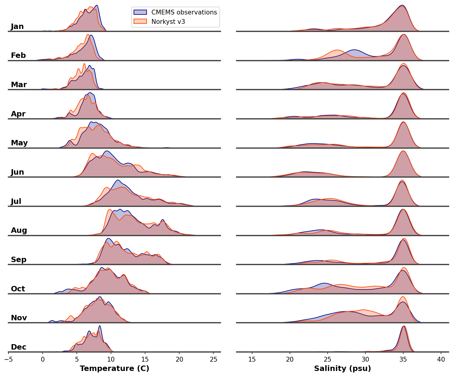
**Figure 2** — Comparison of temperature and salinity distributions in the upper 20 m between the Norkyst v.3 hindcast archive and the gridded CORA dataset (2015–2022). The close agreement in both distributions indicates that the model captures the main environmental conditions and their seasonal variability in the open ocean. *(Christensen et al., 2026, Fig. 2)*#

Systematic biases vary with depth and season. In the surface and upper layers (0–100 m) a slight warm bias appears in early autumn, while a cold bias is present in winter. The intermediate layer (100–250 m) shows a persistent cold bias, whereas the deep layer (>250 m) has a warm bias. These biases are generally small relative to natural variability.

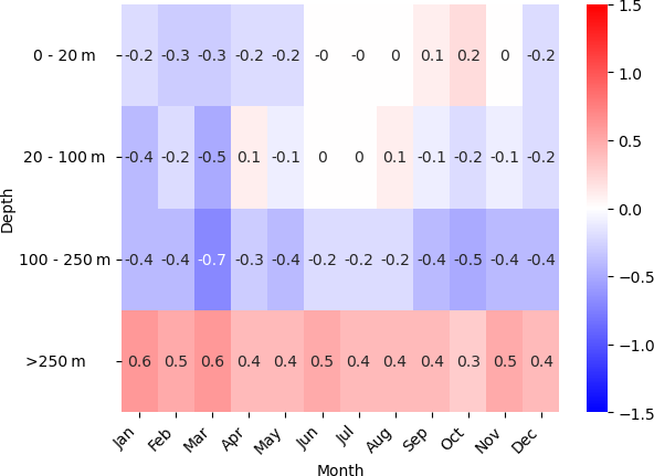
Temperature bias heatmap by month and depth — **Figure 3** — Monthly temperature bias between the Norkyst v.3 hindcast and the CORA dataset (2015–2022), categorised by depth layer. Warm colours indicate a positive (warm) model bias; cool colours a negative (cold) bias. *(Christensen et al., 2026, Fig. 3)*#

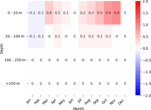
Salinity bias heatmap by month and depth — **Figure 4** — Monthly salinity bias between the Norkyst v.3 hindcast and the CORA dataset (2015–2022), categorised by depth layer. A positive surface salinity bias is present; its attribution among boundary conditions, river discharge, and internal model processes remains an open question. *(Christensen et al., 2026, Fig. 4)*#

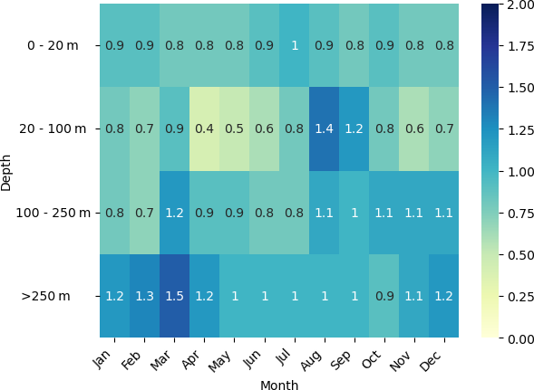
Temperature RMSE heatmap by month and depth — **Figure 5** — Monthly temperature RMSE between the Norkyst v.3 hindcast and the CORA dataset (2015–2022). Errors are generally below 1 °C and are smaller near the surface than at depth. *(Christensen et al., 2026, Fig. 5)*#

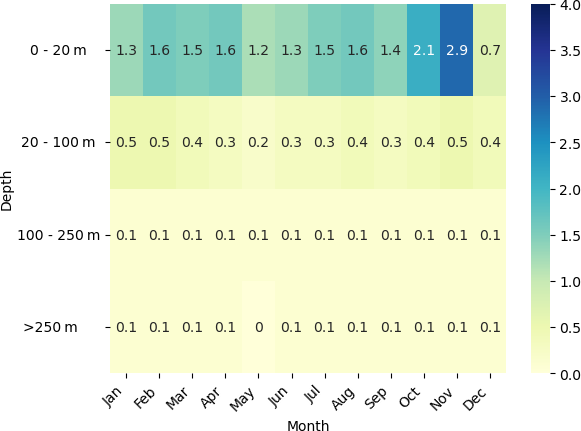
Salinity RMSE heatmap by month and depth — **Figure 6** — Monthly salinity RMSE between the Norkyst v.3 hindcast and the CORA dataset (2015–2022). Salinity observations are sparse below 100 m, but available data indicate small errors at those levels. *(Christensen et al., 2026, Fig. 6)*#

Coastal ocean hydrography#

The coastal zone evaluation uses temperature and salinity profiles from seven IMR fixed coastal stations, spanning from Lista in the south to Ingøy in the north (see Fig. 1 above for station positions), measured 2–4 times per month throughout 2012–2023. Validation focuses on 10 m (surface layer) and 150 m (intermediate layer).

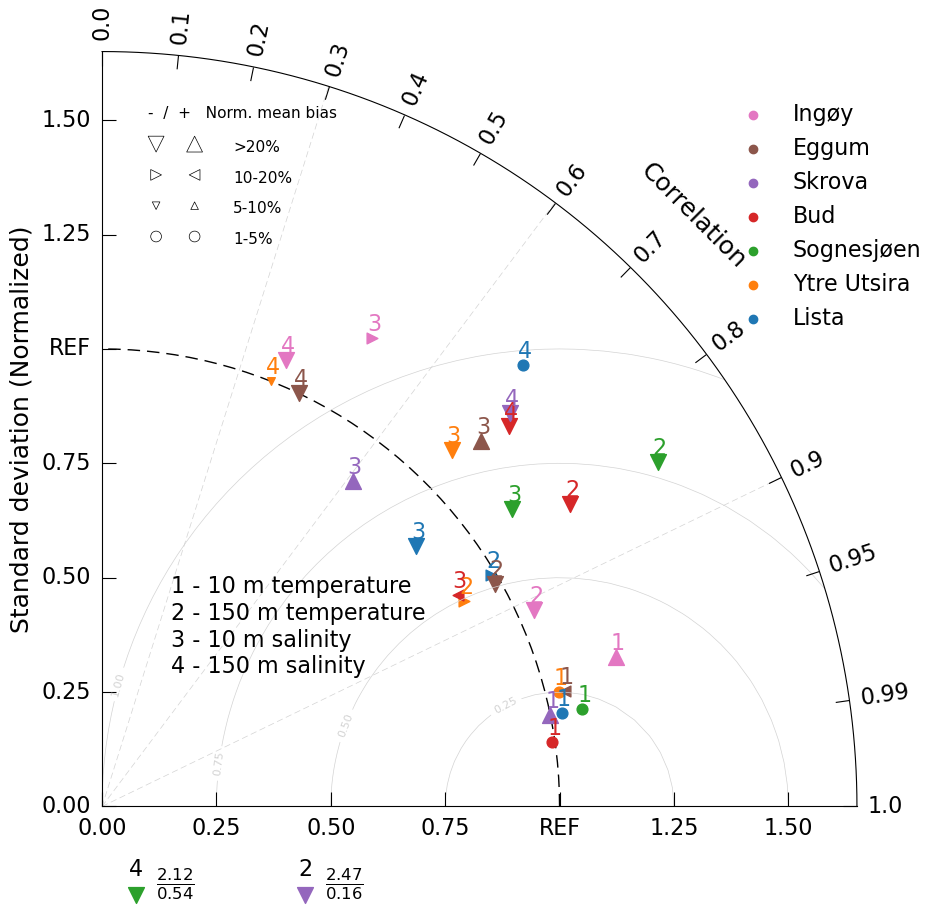
Taylor diagram for coastal hydrographic stations — **Figure 7** — Taylor diagram showing correlation coefficient, normalised standard deviation, RMSE (grey curved lines), and normalised mean bias (symbol type and size) for modelled versus observed temperature and salinity at 10 m and 150 m depth at the seven fixed coastal stations (2012–2023). Colours denote individual stations. *(Christensen et al., 2026, Fig. 7)*#

Surface-layer temperature (10 m) is very well reproduced at all stations, with standard deviations close to observed values and high correlations. Normalised temperature biases are below 5 % at the southernmost stations, and somewhat larger at the northernmost stations. Salinity performance is slightly lower, reflecting the greater spatial variability and sensitivity to river discharge estimates. The complete time series from the station Ytre Utsira (southern Norway) illustrates the high quality of the surface-layer simulation:

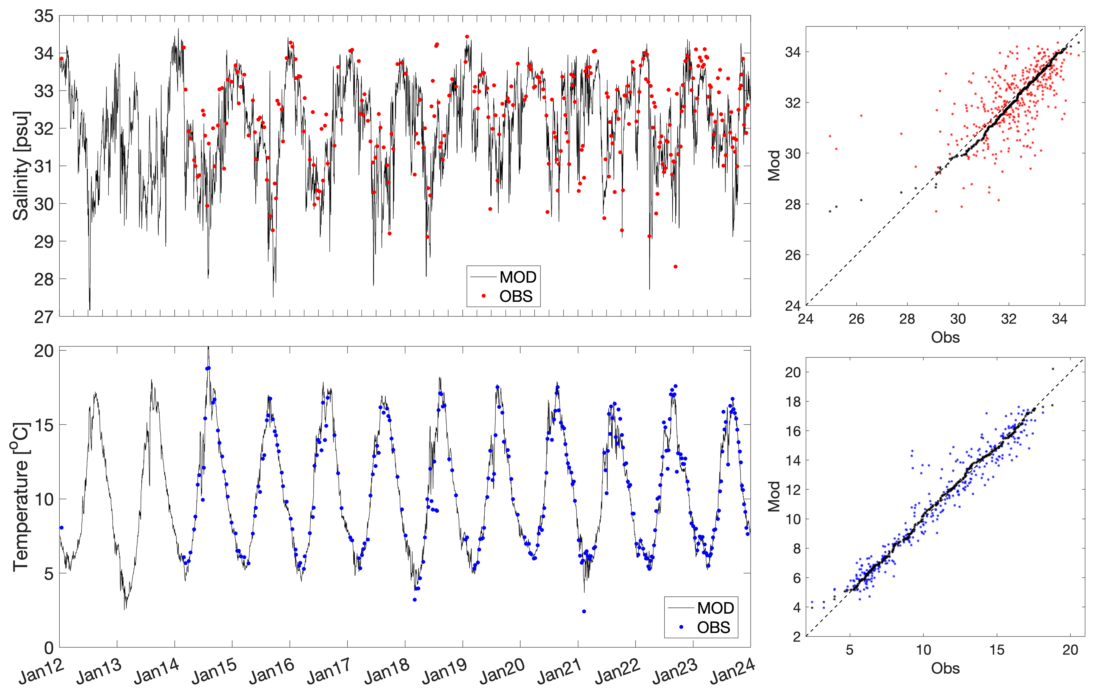
Salinity and temperature time series at Ytre Utsira, 10 m depth — **Figure 8** — Salinity (top) and temperature (bottom) at the fixed station Ytre Utsira at 10 m depth, 2012–2023. Model values are shown as black lines; observed values as coloured dots. Rightmost panels summarise scatter plots, Q–Q plots, and histograms of deviations. *(Christensen et al., 2026, Fig. 8)*#

At 150 m depth, the model generally captures the intermediate-layer variability with realistic standard deviations and high correlations, though with somewhat larger discrepancies than at the surface. The station Skrova (northern Norway) is a challenging location where the model overestimates temperature variability and underestimates salinity:

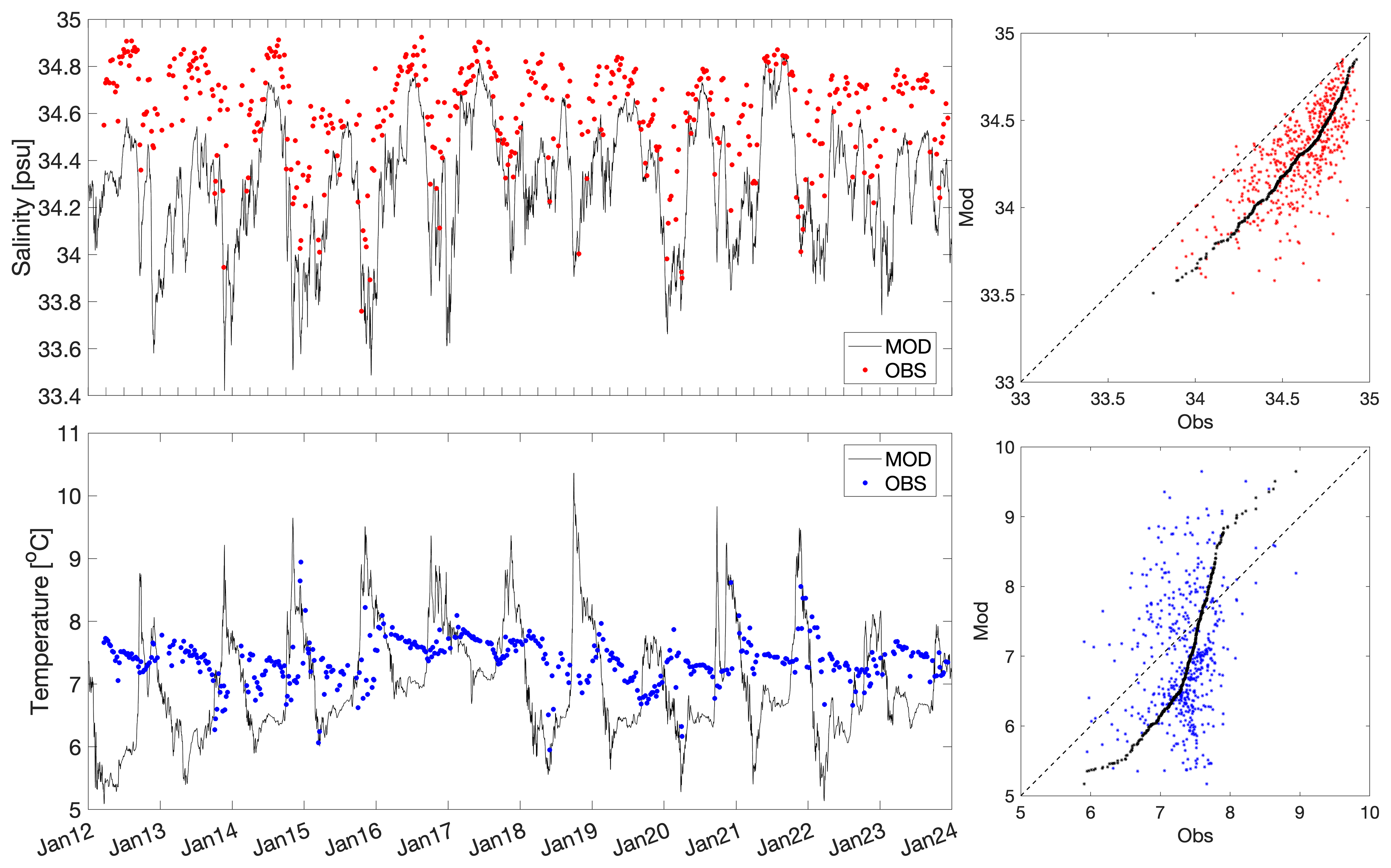
Salinity and temperature time series at Skrova, 150 m depth — **Figure 9** — Same as Figure 8 but from the fixed station Skrova at 150 m depth. *(Christensen et al., 2026, Fig. 9)*#

Fjord circulation — Hardangerfjord#

Norkyst is also evaluated against current measurements and hydrographic profiles from the Hardangerfjord, one of Norway’s largest and deepest fjords (~180 km long, maximum depth ~860 m). Two locations are used:

HfjE (“Hardangerfjord East”): approximately 60 km from the fjord mouth, bottom depth 540 m. Along-fjord currents were measured January–April 2024 at 10, 30 and 100 m depths using two Nortek profiling current meters.
H2: approximately 120 km from the fjord mouth, bottom depth 850 m. Monthly CTD profiles were collected 2017–2023.

At HfjE, episodic in- and outflow events driven by wind, tides and internal pressure gradients are well represented by the model. Using the skill classification of Dalsøren et al. (2020), model results are rated “good” for 78 %, 75 % and 90 % of the time at 10, 30 and 100 m depths respectively.

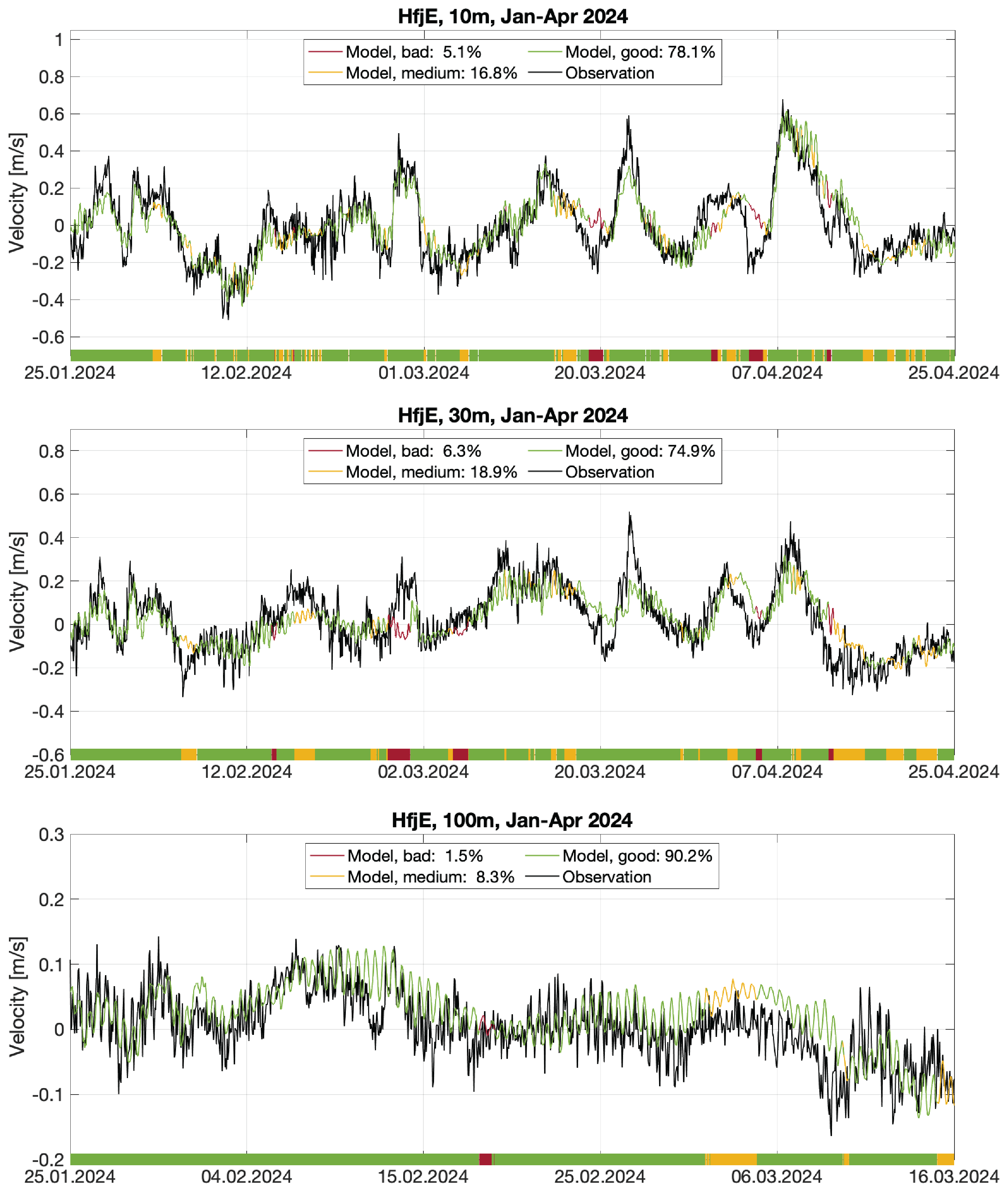
Along-fjord current time series at Hardangerfjord East — **Figure 10** — Along-fjord current from observations (coloured) and Norkyst (grey) at 10, 30 and 100 m depths at Hardangerfjord East, January–April 2024. Categories “good”, “medium” and “bad” follow Dalsøren et al. (2020): “good” implies correct direction and low bias, “medium” correct direction but high bias, and “bad” when the modelled flow direction is wrong. *(Christensen et al., 2026, Fig. 10)*#

At H2, the inner fjord shows a pronounced seasonal surface brackish layer (salinity < 5 at 3 m depth in summer), strong thermal stratification (surface temperature ranging from ~4 °C in winter to ~18 °C in summer), and a phase-shifted deep temperature cycle (warmest in winter, coldest in summer at 100 m depth). The model captures the observed hydrography at 3 m depth with deviations typically less than one unit in both temperature and salinity. At 100 m depth a slight cold and fresh bias is present.

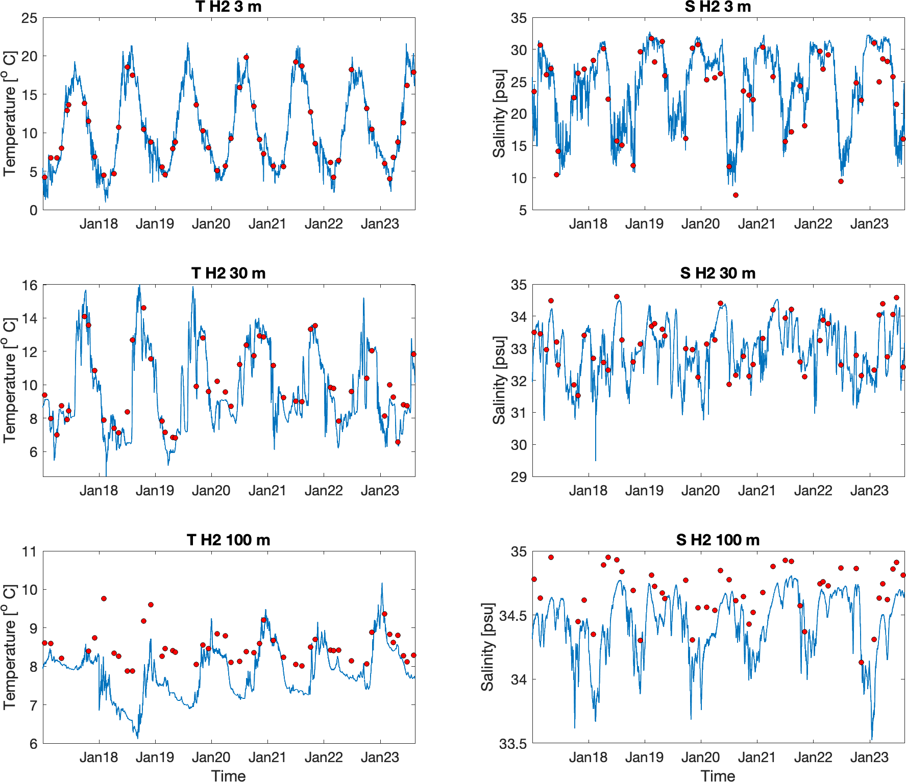
Temperature and salinity time series at H2 in the Hardangerfjord — **Figure 11** — Temperature (left) and salinity (right) at 3, 30 and 100 m depths at location H2 in the inner Hardangerfjord, 2017–2023. Observations are shown as red dots; daily mean Norkyst values as solid blue lines. *(Christensen et al., 2026, Fig. 11)*#

Operational setup and data access#

The operational implementation of Norkyst runs once per day on the high-performance computing infrastructure of MET Norway. Each day, updated boundary data, atmospheric forcing, climatological nudging fields, and river runoff estimates are downloaded and pre-processed before the simulation begins.

Forecast product: The system generates 120 h (5-day) prognoses initialised at 00:00 UTC daily. Output is written in netCDF format, following CF conventions (Eaton et al., 2024) and FAIR principles (Wilkinson et al., 2016). For the operational forecasts, 3D fields are interpolated from the 40 native sigma layers to 15 fixed depth levels (0, 1, 2, 3, 5, 7, 10, 15, 25, 50, 65, 75, 100, 200 and 300 m).
Output variables: Available fields include eastward and northward current components (u_eastward, v_northward, w), salinity, temperature, sea surface elevation (zeta), vertical tracer diffusivity (AKs), and surface wind components (Uwind_eastward, Vwind_northward).
Hindcast archive: A continuously updated hindcast extends back to 2012 and is available on both the native sigma-coordinate grid and interpolated to 25 fixed depth levels. It is updated quarterly and currently covers up to and including December 2024.
Downstream applications: Norkyst output serves as driver data for the OpenDrift trajectory model, used operationally by Norwegian authorities for search-and-rescue, oil drift, and vessel drift applications. Norkyst also supports environmental management services for the aquaculture industry, including estimates of salmon lice transmission and organic loading (Sandvik et al., 2020).

Data and code availability

Resource	Link
5-day forecast archive (hourly)	data.met.no
Hindcast archive (from 2012)	thredds.met.no
API (selected fields)	api.met.no
ROMS configuration files (Zenodo)	doi:10.5281/zenodo.16810677
Analysis and plotting scripts (Zenodo)	doi:10.5281/zenodo.17053760
Full ROMS model code (Zenodo)	doi:10.5281/zenodo.17046086

Ongoing developments#

The Norkyst modeling system is under active development. Current and planned activities include the following:

Data assimilation: A coarser-resolution (2.4 km) version of Norkyst with 4D-Var data assimilation (“Norkyst-DA”) has been operational since 2017. Work is underway to adapt the assimilation scheme to Norkyst v.3, investigating a mixed-resolution, mixed-precision approach with reduced resolution and precision in the inner minimisation loops (Iversen et al., 2023).
Ensemble prediction: To provide downstream users with quantitative uncertainty information, the operational system is configured to support parallel execution of multiple model instances for ensemble prediction.
Two-way nested high-resolution fjord models: ROMS two-way nesting (5:1 refinement, i.e. 160 m horizontal resolution) is used to produce seamless high-resolution simulations of selected fjord systems. Operational nested models currently cover the Oslofjord region and one area of Western Norway (Mørekysten), with further regions planned.
Wave–current coupling: Coupling to surface waves through the virtual wave stress, Coriolis–Stokes force, and wave-breaking turbulence injection has been tested and is under continued development. Operational wave prediction systems already use Norkyst currents to model wave refraction, enabling weak two-way coupling. Improvements to the lateral boundary condition implementation, including bias correction schemes, are also planned.
Sea ice: Although the Norwegian coast is largely ice-free, work is underway to evaluate the suitability of a sea ice model recently integrated with the ROMS version used in Norkyst, targeting occasional winter ice formation in sheltered fjords.