Plot cross-section#

In this notebook, we will see how a cross-section can be created, and how we can extract temperature values from Norkyst along this section.

Python requirements

To access data from the model and extracting it into datasets we will make use of some Python packages. Xarray will be the main tool to opening the datasets, and allows us to display the contents nicely. Cartopy and matplotlib are the main plotting tools, in addition to Cmocean for colormaps. Additionally, we will use pyresample and pyproj to deal with geographical coordinates and their collocation with the model grid.

import numpy as np
import matplotlib.pyplot as plt
from matplotlib.colors import BoundaryNorm, ListedColormap

import cartopy.crs as ccrs
import cartopy.feature as cfeature
from cartopy.mpl.gridliner import LONGITUDE_FORMATTER, LATITUDE_FORMATTER

import cmocean.cm as cmo
import xarray as xr

from pyproj import Geod
import pyresample

We define the path for the target data set here.

YEAR = 2026
MT = str(4).zfill(2) # zero-padded
DAY = str(25).zfill(2)

path = 'https://thredds.met.no/thredds/dodsC/fou-hi/norkystv3_his_files/%i/%s/%s/norkyst800_his_zdepth_%i%s%sT00Z_m00_AN.nc'%(YEAR, MT, DAY, YEAR, MT, DAY)

ds = xr.open_dataset(path)

""
ds

We select now the transect points we want to work on, and make a quick plot of it over the surface temperature values

# The transect we will be working with
lat_sec = np.array([57.95, 57.10]) # start_lat, end_lat
lon_sec = np.array([7.31, 8.41])  # start_lon, end_lon

#lat_sec = np.array([58.50, 57.68]) # start_lat, end_lat
#lon_sec = np.array([9.02, 10.32])  # start_lon, end_lon

# Latitude and longitude of the dataset
lat = ds.lat.values
lon = ds.lon.values

## Make a map of the area with the transect ####

# Choosing a map projection
proj = ccrs.NorthPolarStereo()

# Making figure and axes with the projection
fig, ax = plt.subplots(subplot_kw={'projection': proj}, constrained_layout=True, dpi=200)

# Setting the extent of the map to our model domain
ax.set_extent([np.min(lon), np.max(lon), np.min(lat), np.max(lat)], crs=ccrs.PlateCarree())  # ccrs.PlateCarree() to tell the program our data is in coordinates lats/lons

# Adding natural features to our map
land = cfeature.NaturalEarthFeature(category='physical', name='land', scale='50m', edgecolor='gray', facecolor=cfeature.COLORS['land'])
coastline = cfeature.NaturalEarthFeature(category='physical', name='coastline', scale='50m', edgecolor='gray', facecolor='none')
borders = cfeature.NaturalEarthFeature(category='cultural', name='admin_0_boundary_lines_land', edgecolor= 'gray', scale='50m', facecolor='none')

ax.add_feature(land)
ax.add_feature(coastline)
ax.add_feature(borders)

# Adding gridlines
gl = ax.gridlines(crs=ccrs.PlateCarree(), draw_labels=True, linewidth=1, color='lightgray', alpha=0.5, linestyle='--')
gl.top_labels = False  # Disable top labels
gl.right_labels = False  # Disable right labels
gl.xformatter = LONGITUDE_FORMATTER
gl.yformatter = LATITUDE_FORMATTER

# Plotting boundaries of model
ax.plot(lon[0,:], lat[0,:], '--', transform= ccrs.PlateCarree(), color = 'gray', linewidth =0.8)
ax.plot(lon[-1,:], lat[-1,:], '--', transform= ccrs.PlateCarree(), color = 'gray', linewidth =0.8)
ax.plot(lon[:,0], lat[:,0], '--', transform= ccrs.PlateCarree(), color = 'gray', linewidth =0.8)
ax.plot(lon[:,-1], lat[:,-1], '--', transform= ccrs.PlateCarree(), color = 'gray', linewidth =0.8, label='Norkyst boundary')

# Plotting sea surface height
temp_norkyst = ds.temperature.isel(time=22, depth=0)
cs = temp_norkyst.plot.pcolormesh(ax=ax, x='lon', y='lat', vmin=6, vmax=10, cmap=cmo.thermal, transform=ccrs.PlateCarree())

# Adding transect
ax.plot([lon_sec[0], lon_sec[1]], [lat_sec[0], lat_sec[1]], transform = ccrs.PlateCarree(), color = 'r', label = 'Transect')

# Adding legend
ax.legend(loc = 'upper left')

depth = 0.0 [meter], time = 2026-04-25T22:00:00

<matplotlib.legend.Legend object at 0x7f2308908d70>

The next step now is the extraction of values along the defined transect. We want salinity and temperature values. For that, we have to define a function which will perform the job of xroms.argsel2d.

def generate_transect_points(lat_init, lon_init,
                              lat_end, lon_end,
                              n_points=100):
    """
    Generate evenly spaced points along a geodesic transect.

    Parameters
    ----------
    lat_init, lon_init : float
        Start point coordinates.
    lat_end, lon_end : float
        End point coordinates.
    n_points : int
        Total number of points INCLUDING endpoints.

    Returns
    -------
    lats : ndarray
    lons : ndarray
    """

    geod = Geod(ellps="WGS84")

    # npts excludes endpoints
    intermediate = geod.npts(
        lon_init, lat_init,
        lon_end, lat_end,
        n_points - 2
    )

    # Build full coordinate list
    lons = [lon_init] + [p[0] for p in intermediate] + [lon_end]
    lats = [lat_init] + [p[1] for p in intermediate] + [lat_end]

    return np.array(lats), np.array(lons)

# Here we generate the transect points using the function defined above
lat_t, lon_t = generate_transect_points(lat_sec[0], lon_sec[0], lat_sec[1], lon_sec[1], n_points=100)


# Extract the 2D longitude and latitude arrays from the dataset
lon2d = ds['lon'].values
lat2d = ds['lat'].values


ds_geo = pyresample.geometry.GridDefinition(lons=lon2d, lats=lat2d)
pos_geo = pyresample.geometry.SwathDefinition(lons=lon_t, lats=lat_t)

_, valid_output_index, index_array, distance_array = \
                        pyresample.kd_tree.get_neighbour_info(
                            source_geo_def=ds_geo,
                            target_geo_def=pos_geo,
                            radius_of_influence=800,
                            neighbours=1)

index_array_2d = np.unravel_index(index_array, ds.lon.shape)

# Ensure rows and cols are treated as 1D arrays
rows_da = xr.DataArray(np.array(index_array_2d[0]), dims="points")
cols_da = xr.DataArray(np.array(index_array_2d[1]), dims="points")

# Extract the data for these unique indices
transect_ds = ds.isel(Y=rows_da, X=cols_da)  # Replace 'y' and 'x' with actual dimension names

We use a function here to calculate the cumulative distance along the transect

def compute_transect_distance(lons, lats):
    """
    Compute cumulative distance along transect.

    Parameters
    ----------
    lons, lats : 1D arrays

    Returns
    -------
    distance_km : 1D array
        Cumulative distance in km
    """

    geod = Geod(ellps="WGS84")

    distance_km = np.zeros(len(lons))

    for i in range(1, len(lons)):

        _, _, dist_m = geod.inv(
            lons[i-1], lats[i-1],
            lons[i], lats[i]
        )

        distance_km[i] = distance_km[i-1] + dist_m / 1000

    return distance_km

distance_km = compute_transect_distance(lon_t, lat_t)

""

''

We plot our transaction using a grid interpolator, so the bathymetry contour is properly displayed.

from scipy.interpolate import RegularGridInterpolator

# -----------------------
# INPUT DATA
# -----------------------
temp = transect_ds.temperature[0,:,:].values        # (depth, points)
z = transect_ds.depth.values          # (depth,)
dist = distance_km # (points,)
h = transect_ds.h.values              # (points,)

# -----------------------
# 1. CREATE TARGET GRID
# -----------------------
dist_grid = np.linspace(dist.min(), dist.max(), 300)
z_grid = np.linspace(0, z.max(), 200)

dist2d, z2d = np.meshgrid(dist_grid, z_grid)

# -----------------------
# 2. INTERPOLATOR (structured grid: depth × distance)
# -----------------------
f = RegularGridInterpolator(
    (z, dist),
    temp,
    bounds_error=False,
    fill_value=np.nan
)

# evaluate on grid
points = np.column_stack([z2d.ravel(), dist2d.ravel()])
temp_grid = f(points).reshape(z2d.shape)

# -----------------------
# 3. BATHYMETRY MASK
# -----------------------
# interpolate h onto grid horizontally
h_interp = np.interp(dist_grid, dist, h)

mask = z2d <= h_interp[None, :]
temp_grid[~mask] = np.nan

# -----------------------
# 4. PLOT
# -----------------------
fig, ax = plt.subplots(figsize=(12, 5))

# seabed
ax.fill_between(
    dist_grid,
    z_grid.min(),
    h_interp,
    color="w",
    alpha=0.3,
    ec='k',

)

pcm = ax.pcolormesh(
    dist_grid,
    z_grid,
    temp_grid,
    vmin=6,
    vmax=8,
    cmap=cmo.thermal,
    shading="auto"
)

cb = plt.colorbar(pcm, ax=ax)
cb.set_label(r"Potential temperature [C$^{\degree}$]")

ax.set_xlabel("Distance (km)")
ax.set_ylabel("Depth (m)")
ax.invert_yaxis()
ax.set_title("Interpolated cross-section")

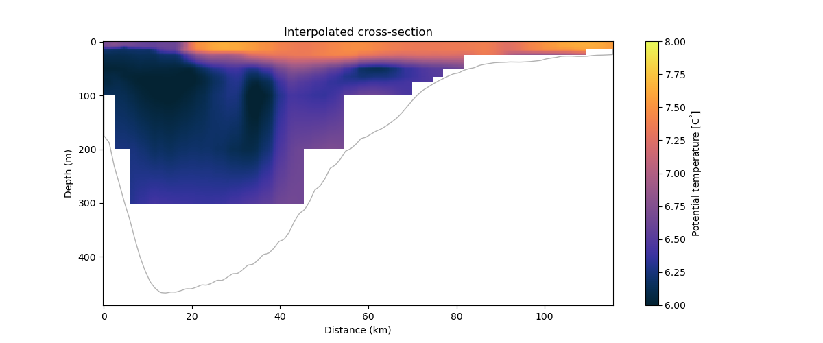
Text(0.5, 1.0, 'Interpolated cross-section')

Cross-section in S-coordinates#

We can also make a plot of the same cross-section using outputs defined in S-coords. The later represents a terrain-following coordinate system, therefore, we must convert the output variables there to true depth values using the following equation:

$$Z_0 = frac{h_c , S + h , C}{h_c + h}$$

$$z = Z_0 (zeta + h) + zeta$$

path_s = './datasets/transect_scoord.nc'
ds_s = xr.open_dataset(path_s, engine='netcdf4')

""

''

Employ the conversion here:

Zo_rho = (ds_s.hc * ds_s.s_rho + ds_s.Cs_r * ds_s.h) / (ds_s.hc + ds_s.h)
z_rho = ds_s.zeta + (ds_s.zeta + ds_s.h) * Zo_rho

ds_s.coords["z_rho"] = z_rho.transpose()

You can have a quick look at the results using:

section = ds_s.temp
section.plot(x="lon_rho", y="z_rho", figsize=(15, 6), clim=(6, 8), cmap=cmo.thermal)
plt.ylim([-500, 1]);

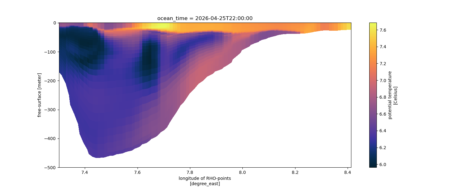
(-500.0, 1.0)

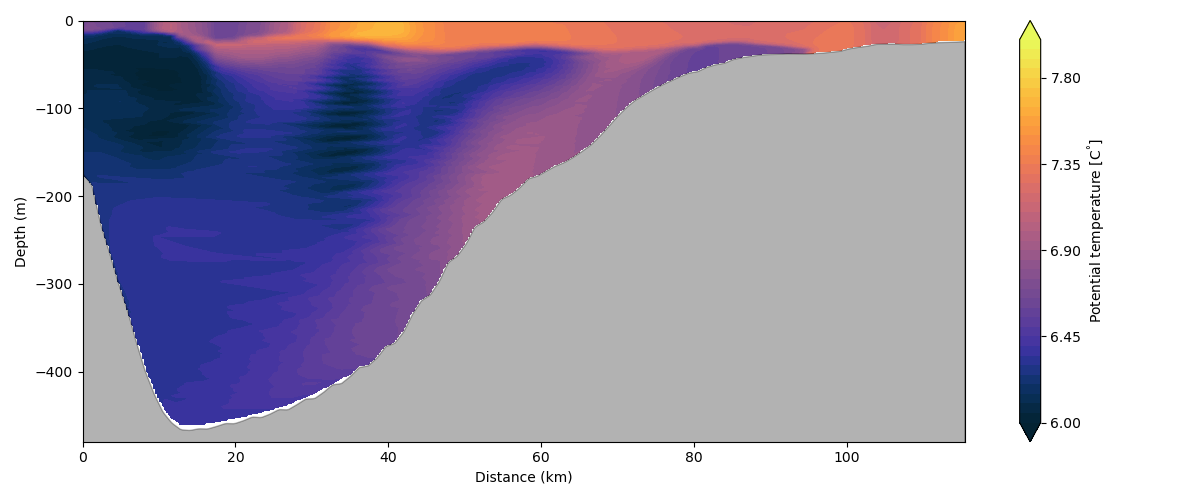
Or, plot it using Matplotlib if you want more control over your options:

from scipy.interpolate import griddata

# -----------------------------------
# SELECT TIME
# -----------------------------------

temp = ds_s.temp.values
# shape: (40, 100)

# -----------------------------------
# DISTANCE
# -----------------------------------

dist = distance_km
# shape: (100,)

# -----------------------------------
# TRUE DEPTHS
# -----------------------------------
z_rho = ds_s.z_rho.values

# -----------------------------------
# BUILD SCATTERED POINTS
# -----------------------------------

dist2d = np.tile(dist, (temp.shape[0], 1))

points = np.column_stack([
    dist2d.ravel(),
    z_rho.ravel()
])

values = temp.ravel()

# remove NaNs
mask = np.isfinite(values) & np.isfinite(points[:,1])

points = points[mask]
values = values[mask]

# -----------------------------------
# TARGET GRID
# -----------------------------------

dist_grid = np.linspace(dist.min(), dist.max(), 400)

z_grid = np.linspace(
    np.nanmin(z_rho),
    0,
    300
)

distg, zg = np.meshgrid(dist_grid, z_grid)

# -----------------------------------
# INTERPOLATE
# -----------------------------------

temp_grid = griddata(
    points,
    values,
    (distg, zg),
    method="linear"
)

# -----------------------------------
# BATHYMETRY
# -----------------------------------

h = -transect_ds.h.values

h_grid = np.interp(
    dist_grid,
    dist,
    h
)

# mask below seafloor
temp_grid[zg < h_grid[None, :]] = np.nan

# -----------------------------------
# PLOT
# -----------------------------------

fig, ax = plt.subplots(figsize=(12,5))

pcm = ax.contourf(
    distg,
    zg,
    temp_grid,
    levels=np.linspace(6, 8, 41),
    shading="auto",
    cmap=cmo.thermal,
    extend="both"
)

# Define colorbar
cbar = plt.colorbar(pcm, ax=ax, label=r"Potential temperature [C$^{\degree}$]")
cbar.ax.locator_params(nbins=5)


# fill land
ax.fill_between(
    dist_grid,
    h_grid,
    zg.min()-20,
    color="k",
    alpha=0.3
)

# Set labels
ax.set_ylim(-480, 0)
ax.set_xlabel("Distance (km)")
ax.set_ylabel("Depth (m)")

plt.tight_layout()
plt.show()

/home/runner/work/norkyst.github.io/norkyst.github.io/examples/example_cross.py:409: UserWarning: The following kwargs were not used by contour: 'shading'
  pcm = ax.contourf(

Total running time of the script: (0 minutes 39.863 seconds)

Gallery generated by Sphinx-Gallery