Note
Go to the end to download the full example code.
Calculate and plot Turner Angle#
Here we illustrate how to extract data on the native ROMS model grid, and to plot the statistics of the vertical distribution of the so-called Turner angle. The Turner angle was proposed by Ruddick [1], and is defined as
\(\mathrm{Tu} = \tan^{-1}\left( \alpha \frac{\partial \theta}{\partial z} - \beta \frac{\partial S}{\partial z}, \alpha \frac{\partial \theta}{\partial x} - \beta \frac{\partial S}{\partial x} \right)\) where \(\theta\) is the potential temperature, \(S\) is the salinity, \(\alpha\) is the thermal expansion coefficient, and \(\beta\) is the haline contraction coefficient. The Turner angle can be used to investigate the stability of a water column, and the separate roles of salinity and temperature for this stability. It is related to the density ratio, but is perhaps generally more useful for diagnostics. The Wikipedia page is informative, and as they say there, the most relevant ranges are:
If −45° < Tu < 45°, the column is statically stable.
If −90° < Tu < −45°, the column is unstable to diffusive convection.
If 45° < Tu < 90°, the column is unstable to salt fingering.
If −90° > Tu or Tu > 90°, the column is statically unstable to Rayleigh–Taylor instability (Unstable).
In this notebook we will be fetching a subset of the full output file and plot the median vertical distribution of the Turner angle in addition to the 5, 25, 75, and 95 percentiles. A plot is made highlighting the different regimes listed above. Note that our code uses the gsw package that is based on TEOS-10, and hence we do a conversion inside the tad function called below from potential temperature and practical salinity to conservative temperature and absolute salinity.
[1]: Ruddick, B. (1983), “A practical indicator of the stability of the water column to double-diffusive activity”, _Deep Sea Res._, 30, pp. 1105-1107.
import numpy as np
import matplotlib.pyplot as plt
from matplotlib.colors import BoundaryNorm, ListedColormap

import cmocean.cm as cmo
import xarray as xr
import gsw

from scipy.interpolate import griddata
from pyproj import Geod
from scipy.interpolate import interp1d

# Load the dataset and resample to daily means
ds = xr.open_dataset('./datasets/timeseries_norkyst_2025_deep.nc', engine='netcdf4').resample(ocean_time="D").mean(dim="ocean_time")
ds = ds.isel(s_rho=slice(None, None, -1)) # Invert the vertical coordinate to have depth increasing downwards

# ---------------------------------------- #
# --- Conversion from S-coord to depth --- #
# ---------------------------------------- #
Zo_rho = (ds.hc * ds.s_rho + ds.Cs_r * ds.h) / (ds.hc + ds.h)
z_rho = ds.zeta + (ds.zeta + ds.h) * Zo_rho

ds.coords["z_rho"] = z_rho.transpose('ocean_time', 's_rho')

# ----------------------------------------------------------------------- #
# --- Convert salinity and temperature from ROMS to TEOS-10 standards --- #
# ----------------------------------------------------------------------- #
salt = ds.salt
temp = ds.temp
Convert temperature and salinity#
maxdepth = -450.0
resolution = 200
# Interpolate to fixed depths
zout = np.linspace(maxdepth,-1,resolution)
# Convert salinity and temperature from ROMS to TEOS-10 standards
p = gsw.conversions.p_from_z(ds.z_rho, 57.5) # Lat
SA = gsw.conversions.SA_from_SP(salt, p, 8, 57.5) # Lon, Lat
CT = gsw.conversions.CT_from_pt(SA, temp)
rho0 = gsw.pot_rho_t_exact(SA, CT, p, 0) # Ref level
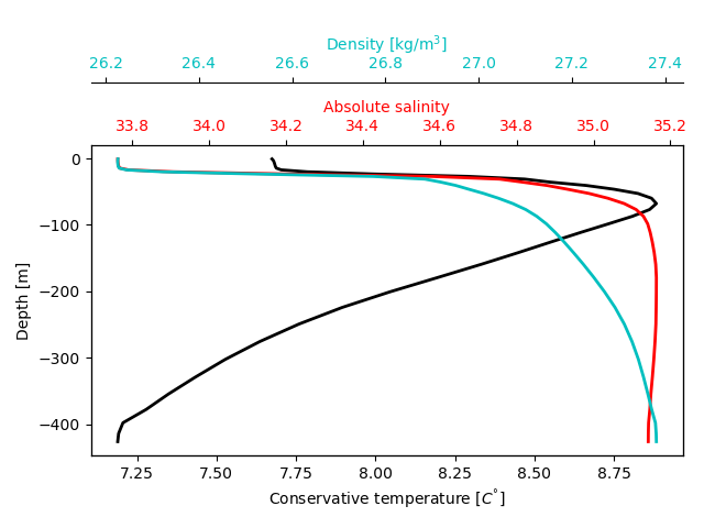
# ------------------------------------------------ #
# --- Plot vertical profile of SA, CT, and rh0 --- #
# ------------------------------------------------ #
index = 0
fig, ax1 = plt.subplots()
#plt.scatter(Tu_angle[index,:], zout, label='Tu')
ax1.plot(CT[index,:], ds.z_rho[index,:], c='k', lw=2);
ax1.set_xlabel(r'Conservative temperature $[C^{\degree}]$', color='k')
ax1.set_ylabel('Depth [m]', color='k')
ax2 = ax1.twiny() # instantiate a second Axes that shares the same x-axis
ax2.set_xlabel('Absolute salinity', color='r')
ax2.plot(SA[index,:], ds.z_rho[index,:], c='r', lw=2);
ax2.tick_params(axis='x', labelcolor='r')
fig.tight_layout()
ax3 = ax1.twiny() # instantiate a second Axes that shares the same x-axis
ax3.spines["top"].set_position(("axes", 1.2))
ax3.set_xlabel(r'Density $[\text{kg/m}^{3}]$', color='c')
ax3.plot(rho0[index,:] - 1000, ds.z_rho[index,:], c='c', lw=2);
ax3.tick_params(axis='x', labelcolor='c')
fig.tight_layout()
Calculate Turner Angle#
# Declare empty arrays for Turner angle
Tu_angle = np.zeros((SA.shape[0], len(zout)))
N2 = np.zeros((SA.shape[0], len(zout)))

for i in range(SA.shape[0]):

    # Get Turner angle
    Tu, Rs, pmid = gsw.Turner_Rsubrho(SA[i,:],CT[i,:],p[i,:])
    z = gsw.z_from_p(pmid, 57.5)
    f = interp1d(z, Tu, bounds_error=False, fill_value=np.nan)

    n2, pmid = gsw.Nsquared(SA[i,:], CT[i,:], p[i,:], lat=57.5)
    f_n2 = interp1d(gsw.z_from_p(pmid, 57.5), n2, bounds_error=False, fill_value=np.nan)

    Tu_angle[i,:] = f(zout)
    N2[i,:] = f_n2(zout)
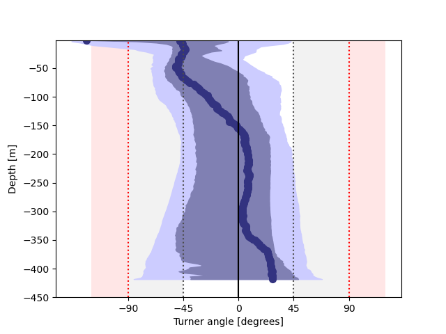
Plot the quartiles#
# Loop over levels and compute percentiles
tu = np.zeros((zout.shape[0],5))

for i in range(len(zout)):
    tu_vals = Tu_angle[:,i].ravel()
    tu[i,:] = np.nanquantile(tu_vals, [0.05,0.25,0.50,0.75,0.95])

# Mark out the four regimes listed above
plt.axvspan(-120, -90, facecolor=[1.0, 0.9, 0.9])
plt.axvspan(-90, -45, facecolor='0.95')
plt.axvspan(45, 90, facecolor='0.95')
plt.axvspan(90, 120, facecolor=[1.0, 0.9, 0.9])

# Plot percentiles and median profiles
plt.fill_betweenx(zout, tu[:,0], tu[:,4], color=[0.8, 0.8, 1.0])
plt.fill_betweenx(zout, tu[:,1], tu[:,3], color=[0.5, 0.5, 0.7])
plt.scatter(tu[:,2], zout, color=[0.2, 0.2, 0.5], linewidth = 2)

# Delineate regimes for increased clarity
plt.plot([0,0],[maxdepth, 0],'k-')
plt.plot([-45,-45],[maxdepth, 0], color='0.3', linestyle=':')
plt.plot([45,45],[maxdepth, 0], color='0.3', linestyle=':')
plt.plot([-90,-90],[maxdepth, 0],'r:')
plt.plot([90,90],[maxdepth, 0],'r:')

# Set limits, ticks, and labels

plt.ylim((maxdepth, -1))
plt.xticks([-90, -45, 0, 45, 90])
plt.xlabel('Turner angle [degrees]')
plt.ylabel('Depth [m]')
/home/runner/micromamba/envs/norkyst/lib/python3.14/site-packages/numpy/lib/_nanfunctions_impl.py:1573: RuntimeWarning: All-NaN slice encountered
  return _nanquantile_unchecked(

Text(26.472222222222214, 0.5, 'Depth [m]')
Classify results by depth#
import pandas as pd

# --- 1. Turner angle classification ---
classes = np.full(Tu_angle.shape, np.nan, dtype=object)

classes[(Tu_angle >= -45) & (Tu_angle <= 45)] = 'D.S'   # Doubly Stable
classes[(Tu_angle < -45) & (Tu_angle >= -90)] = 'D-C'   # Diffusive Convection
classes[(Tu_angle > 45) & (Tu_angle <= 90)] = 'S.F'     # Salt Fingering
classes[(Tu_angle > 90) | (Tu_angle < -90)] = 'U'   # Unstable

# --- 2. Expand depth to match (time, depth) ---
depth_2d = np.broadcast_to(zout, Tu_angle.shape)

# --- 3. Flatten consistently ---
depth_flat = depth_2d.ravel()
class_flat = classes.ravel()

# --- 4. Mask invalid values ---
mask = np.isfinite(depth_flat) & pd.notna(class_flat)

depth_flat = depth_flat[mask]
class_flat = class_flat[mask]

# --- 5. Build dataframe ---
df = pd.DataFrame({
    "depth": np.abs(depth_flat),
    "class": class_flat
})

# --- 6. Depth bins ---
bins = [0, 20, 50, 100, 150, 200, 250, 300, 350, 400, 450]

df["depth_bin"] = pd.cut(
    df["depth"],
    bins=bins,
    include_lowest=True
)

# --- 7. Count occurrences ---
# counts (already computed)
counts = pd.crosstab(df["depth_bin"], df["class"])

# percentage of total points (full table)
counts_percent = 100 * counts / counts.to_numpy().sum()

print("=== Percent per depth bin ===")
print(counts_percent)

# --- total percentage per class ---
total_percent_class = 100 * counts.sum(axis=0) / counts.to_numpy().sum()

print("\n=== Total percent per class ===")
print(total_percent_class)
=== Percent per depth bin ===
class                D-C        D.S       S.F         U
depth_bin
(-0.001, 20.0]  1.725236   2.111748  0.037022  0.453152
(20.0, 50.0]    3.856235   3.126157  0.000000  0.044427
(50.0, 100.0]   5.114991   6.769144  0.007404  0.000000
(100.0, 150.0]  2.055474  10.287737  0.088853  0.000000
(150.0, 200.0]  1.049950  10.533564  0.308025  0.000000
(200.0, 250.0]  1.451271   9.859760  0.580509  0.000000
(250.0, 300.0]  2.378308   8.660240  0.852992  0.000000
(300.0, 350.0]  3.238705   7.604366  1.048470  0.000000
(350.0, 400.0]  3.139485   7.333363  1.411287  0.007404
(400.0, 450.0]  1.054393   2.527878  1.101782  0.180668

=== Total percent per class ===
class
D-C    25.064048
D.S    68.813956
S.F     5.436344
U       0.685652
dtype: float64
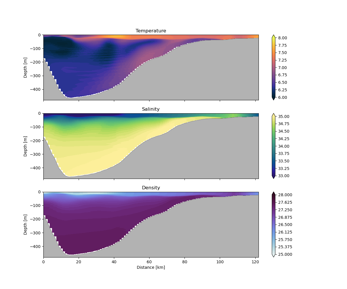
Turner Angle Cross-Section#
We calculate here the Turner Angle for the cross-section used in Cross-section notebook.
path_s = './datasets/transect_scoord.nc'
ds_s = xr.open_dataset(path_s, engine='netcdf4')

Zo_rho = (ds_s.hc * ds_s.s_rho + ds_s.Cs_r * ds_s.h) / (ds_s.hc + ds_s.h)
z_rho = ds_s.zeta + (ds_s.zeta + ds_s.h) * Zo_rho

ds_s.coords["z_rho"] = z_rho.transpose()

# Convert salinity and temperature from ROMS to TEOS-10 standards
p = gsw.conversions.p_from_z(ds_s.z_rho, 57.5) # Lat
SA = gsw.conversions.SA_from_SP(ds_s.salt, p, 8, 57.5) # Lon, Lat
CT = gsw.conversions.CT_from_pt(SA, ds_s.temp)
rho0 = gsw.pot_rho_t_exact(SA, CT, p, 0) # Ref level
Plot temperature along the cross-section#
def compute_transect_distance(lons, lats):
    """
    Compute cumulative distance along transect.

    Parameters
    ----------
    lons, lats : 1D arrays

    Returns
    -------
    distance_km : 1D array
        Cumulative distance in km
    """

    geod = Geod(ellps="WGS84")

    distance_km = np.zeros(len(lons))

    for i in range(1, len(lons)):

        _, _, dist_m = geod.inv(
            lons[i-1], lats[i-1],
            lons[i], lats[i]
        )

        distance_km[i] = distance_km[i-1] + dist_m / 1000

    return distance_km

def interpolate_section(var, z_rho, dist, h,
                        nx=100, nz=400,
                        method="linear"):

    # Build scattered points
    dist2d = np.tile(dist, (var.shape[0], 1))

    points = np.column_stack([
        dist2d.ravel(),
        z_rho.ravel()
    ])

    values = var.ravel()

    # Remove NaNs
    mask = np.isfinite(values) & np.isfinite(points[:, 1])

    points = points[mask]
    values = values[mask]

    # Target grid
    dist_grid = np.linspace(dist.min(), dist.max(), nx)

    z_grid = np.linspace(
        np.nanmin(z_rho),
        0,
        nz
    )

    distg, zg = np.meshgrid(dist_grid, z_grid)

    # Interpolate
    var_grid = griddata(
        points,
        values,
        (distg, zg),
        method=method
    )

    # Bathymetry
    h_grid = np.interp(
        dist_grid,
        dist,
        -h
    )

    # Mask below bottom
    var_grid[zg < h_grid[None, :]] = np.nan

    return distg, zg, var_grid, dist_grid, h_grid

distance_km = compute_transect_distance(ds_s.lon_rho.values, ds_s.lat_rho.values)

z_rho = ds_s.z_rho.values
h = ds_s.h.values

distg, zg, temp_grid, dist_grid, h_grid = interpolate_section(
    ds_s.temp.values,
    z_rho,
    distance_km,
    h
)

_, _, salt_grid, _, _ = interpolate_section(
    ds_s.salt.values,
    z_rho,
    distance_km,
    h
)

_, _, dens_grid, _, _ = interpolate_section(
    rho0.values - 1000,
    z_rho,
    distance_km,
    h
)

fig, axes = plt.subplots(
    3, 1,
    figsize=(12, 10),
    sharex=True
)

fields = [
    (temp_grid, cmo.thermal, np.linspace(6, 8, 41), "Temperature"),
    (salt_grid, cmo.haline,  np.linspace(33, 35, 41), "Salinity"),
    (dens_grid, cmo.dense,   np.linspace(25, 28, 41), "Density")
]

for ax, (field, cmap, levels, title) in zip(axes, fields):

    pcm = ax.contourf(
        distg,
        zg,
        field,
        levels=levels,
        cmap=cmap,
        extend="both"
    )

    ax.fill_between(
        dist_grid,
        h_grid,
        zg.min() - 20,
        color="k",
        alpha=0.3
    )

    ax.set_title(title)
    ax.set_ylim(-480, 0)

    plt.colorbar(pcm, ax=ax)

axes[0].set_ylabel("Depth [m]")
axes[1].set_ylabel("Depth [m]")


axes[-1].set_xlabel("Distance [km]")
axes[-1].set_ylabel("Depth [m]")
Text(96.47222222222221, 0.5, 'Depth [m]')
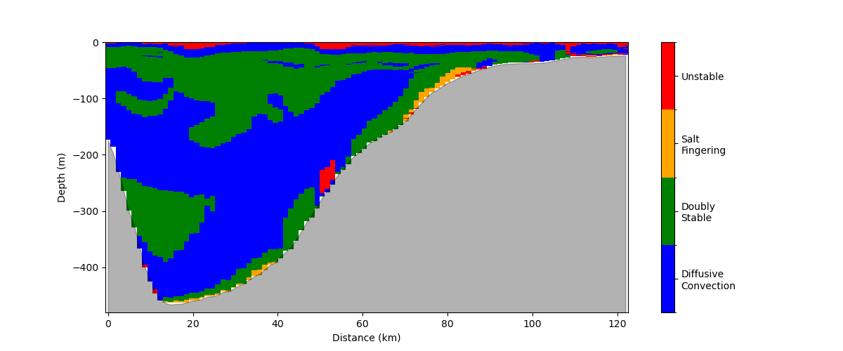
Calculate Turner Angle for the cross-section#
maxdepth = -450.0
resolution = 400

# Interpolate to fixed depths
zout = np.linspace(maxdepth,-1,resolution)

# Convert salinity and temperature from ROMS to TEOS-10 standards
p = gsw.conversions.p_from_z(ds_s.z_rho[::-1,:], 57.5) # Lat
SA = gsw.conversions.SA_from_SP(ds_s.salt.values[::-1,:], p, 8, 57.5) # Lon, Lat
CT = gsw.conversions.CT_from_pt(SA, ds_s.temp.values[::-1,:])

# Declare empty arrays for Turner angle
Tu_angle = np.zeros((SA.shape[1], len(zout)))

for i in range(SA.shape[1]):

    # Get Turner angle
    Tu, Rs, pmid = gsw.Turner_Rsubrho(SA[:, i],CT[:, i],p[:, i])
    z = gsw.z_from_p(pmid, 57.5)

    f = interp1d(z, Tu, bounds_error=False, fill_value=np.nan)
    Tu_angle[i,:] = f(zout)
Plot Turner Angle across the transect#
from matplotlib.colors import ListedColormap, BoundaryNorm

fig, ax = plt.subplots(figsize=(12,5))

# Create regime array
regime = np.full(Tu_angle.shape, np.nan)

# Codes:
# 0 = Diffusive Convection (blue)
# 1 = Statically Stable (green)
# 2 = Salt Fingering (orange)
# 3 = Rayleigh-Taylor (red)

regime[(-90 <= Tu_angle) & (Tu_angle < -45)] = 0 # D-C
regime[(-45 <= Tu_angle) & (Tu_angle <= 45)] = 1 #S.S
regime[(45 < Tu_angle) & (Tu_angle <= 90)] = 2 #S.F
regime[(Tu_angle < -90) | (Tu_angle > 90)] = 3 #R-T


cmap = ListedColormap([
    'blue',    # Diffusive Convection
    'green',   # Statically Stable
    'orange',  # Salt Fingering
    'red'      # Rayleigh-Taylor
])

norm = BoundaryNorm(
    boundaries=[-0.5, 0.5, 1.5, 2.5, 3.5],
    ncolors=cmap.N
)

pcm = ax.pcolormesh(
    distg,
    zg,
    regime.T,
    cmap=cmap,
    norm=norm,
    shading='auto'
)

# fill land
ax.fill_between(
    dist_grid,
    h_grid,
    zg.min()-20,
    color="k",
    alpha=0.3
)


cbar = plt.colorbar(
    pcm,
    ax=ax,
    ticks=[0, 1, 2, 3]
)

cbar.ax.set_yticklabels([
    'Diffusive\nConvection',
    'Doubly\nStable',
    'Salt\nFingering',
    'Unstable'
])

ax.set_ylim(-480, 0)
ax.set_xlabel("Distance (km)")
ax.set_ylabel("Depth (m)")


plt.show()
Total running time of the script: (0 minutes 2.395 seconds)