Plot current maps#

This notebook will give instructions on how to visualize data from the regional ocean model Norkyst, specifically plotting data on maps using Cartopy. The data are retrieved from MET’s THREDDS server. https://thredds.met.no/thredds/catalog.html

Python requirements

To access data from the model and extracting it into datasets we will make use of some Python packages. Xarray will be the main tool to opening the datasets, and allows us to display the contents nicely. Cartopy and matplotlib are the main plotting tools, in addition to Cmocean for colormaps.

If you are unfamiliar with these packages or need help, please see the documentations listed below.

Useful documentation:

Cartopy: https://scitools.org.uk/cartopy/docs/latest/
Cmocean: https://matplotlib.org/cmocean/
Matplotlib: https://matplotlib.org/stable/
NumPy: https://numpy.org/doc/
Xarray:https://docs.xarray.dev/en/stable/

import numpy as np
import pandas as pd
import matplotlib.pyplot as plt
from matplotlib.colors import BoundaryNorm, ListedColormap

import cartopy.crs as ccrs
import cartopy.feature as cfeature
from cartopy.mpl.gridliner import LONGITUDE_FORMATTER, LATITUDE_FORMATTER

import cmocean.cm as cmo
import xarray as xr

import matplotlib
matplotlib.use('Agg')  # Use the Agg backend for rendering

Accessing the data Data can be found at https://thredds.met.no/thredds/catalog.html.

Locate project, folder and files. Here we will use OPENDAP url to read in the data. To get the OPENDAP URL, click on the desired NetCDF file (.nc). Under the “ACCESS” section, select the OPENDAP URL and then copy the URL located under “DATA URL”.

path = 'https://thredds.met.no/thredds/dodsC/fou-hi/norkystv3_his_files/2025/07/24/norkyst800_his_zdepth_20250724T00Z_m00_AN.nc'

ds = xr.open_dataset(path)

""
ds

Plotting data on maps#

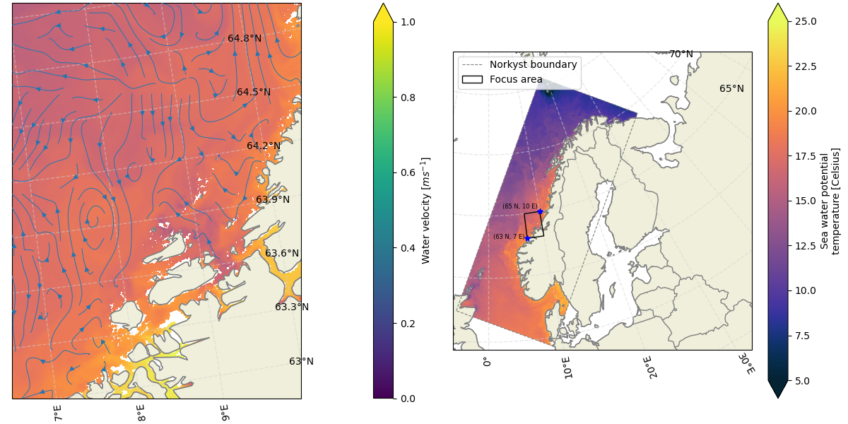
In this example we will plot an excerpt of the model, projected on a map using Cartopy. In Cartopy, the projection determines what the map will look like while the transformaion tells the program which coordinate system your data is in. Our data is in longitude and latitude, so the transformation argument in the plotting function should be: transform=ccrs.PlateCarree(). Matplotlib is the main tool for plotting, but we will make use of cmocean for the color schemes.

The example below shows how to plot the potential temperature and streamlines for currents in an area of the model, with an overview map to it’s right.

# Defining a focus area to plot
lat_area = [65, 63, 63, 65, 65]
lon_area = [7, 7, 10, 10, 7]

""
# Time and depth indices
time_idx = 0
depth_idx = 0

""
# Grid coordinates
lat = ds.lat.values
lon = ds.lon.values

# Current velocity components
u = ds.u_eastward.isel(time=time_idx, depth=depth_idx)
v = ds.v_northward.isel(time=time_idx, depth=depth_idx)

""
fig, axs = plt.subplots(1, 2, figsize=(12, 6), subplot_kw={'projection':ccrs.NorthPolarStereo()}, constrained_layout=True)

# Set the extent of the axes
axs[0].set_extent([np.min(lon_area), np.max(lon_area), np.min(lat_area), np.max(lat_area)], crs=ccrs.PlateCarree())  # This will show our focus area
axs[1].set_extent([np.min(ds.lon.values), np.max(ds.lon.values), np.min(ds.lat.values), np.max(ds.lat.values)], crs=ccrs.PlateCarree())  # This will show an overview

# Add natural features
land = cfeature.NaturalEarthFeature(category='physical', name='land', scale='10m', edgecolor='gray', facecolor=cfeature.COLORS['land'])
coastline = cfeature.NaturalEarthFeature(category='physical', name='coastline', scale='10m', edgecolor='gray', facecolor='none')

axs[0].add_feature(land)
axs[0].add_feature(coastline)

# As the overview map shows a larger area, we can use a coarser resolution for the land/coastline
land = cfeature.NaturalEarthFeature(category='physical', name='land', scale='50m', edgecolor='gray', facecolor=cfeature.COLORS['land'])
coastline = cfeature.NaturalEarthFeature(category='physical', name='coastline', scale='50m', edgecolor='gray', facecolor='none')
borders = cfeature.NaturalEarthFeature(category='cultural', name='admin_0_boundary_lines_land', edgecolor= 'gray', scale='50m', facecolor='none')

axs[1].add_feature(land)
axs[1].add_feature(coastline)
axs[1].add_feature(borders)

# Add gridlines
for ax in axs:
    gl = ax.gridlines(crs=ccrs.PlateCarree(), draw_labels=True, linewidth=1, color='lightgray', alpha=0.5, linestyle='--')
    gl.top_labels = False  # Disable top labels
    gl.right_labels = False  # Disable right labels
    gl.xformatter = LONGITUDE_FORMATTER
    gl.yformatter = LATITUDE_FORMATTER

# Map 1
# Potential temperature field
ds.temperature.isel(time=time_idx, depth=depth_idx).plot(ax=axs[0], x='lon', y='lat', transform=ccrs.PlateCarree(), vmin=5, vmax=25, cmap=cmo.thermal, add_colorbar=False)

# Plot streamlines
sp = axs[0].streamplot(lon, lat, u, v, transform=ccrs.PlateCarree(), cmap=cmo.speed, linewidth=0.7, zorder=5)

# Adding colorbar for the streamlines
cbar = plt.colorbar(sp.lines, ax=axs[0], orientation='vertical', pad=0.2, extend='max', label='Water velocity $[ms^{-1}]$')

# Map 2
# Plotting the boundaries of the model
axs[1].plot(lon[0,:], lat[0,:], '--', transform= ccrs.PlateCarree(), color = 'gray', linewidth =0.8)
axs[1].plot(lon[-1,:], lat[-1,:], '--', transform= ccrs.PlateCarree(), color = 'gray', linewidth =0.8)
axs[1].plot(lon[:,0], lat[:,0], '--', transform= ccrs.PlateCarree(), color = 'gray', linewidth =0.8)
axs[1].plot(lon[:,-1], lat[:,-1], '--', transform= ccrs.PlateCarree(), color = 'gray', linewidth =0.8, label='Norkyst boundary')

# Plot temperature field
temp_norkyst = ds.temperature.isel(time=time_idx, depth=depth_idx)
cs = temp_norkyst.plot.pcolormesh(ax=axs[1], x='lon', y='lat', vmin=5, vmax=25, cmap=cmo.thermal, transform=ccrs.PlateCarree())

# Add box to mark the area plotted in the first map
axs[1].fill(lon_area, lat_area, transform=ccrs.PlateCarree(), color='none', edgecolor='black', linewidth=1, label='Focus area', zorder=10)

# Add markers
axs[1].plot(lon_area[2], lat_area[0], transform = ccrs.PlateCarree(), color = 'blue', marker ='*', markersize=6, zorder=10) # blue stars
axs[1].plot(lon_area[0], lat_area[1], transform = ccrs.PlateCarree(), color = 'blue', marker ='*', markersize=6, zorder=10)

# Add text
axs[1].text(lon_area[2] - 0.25, lat_area[0] + 0.25, '(65 N, 10 E)', horizontalalignment='right', transform=ccrs.PlateCarree(), color = 'black', fontsize = 6)
axs[1].text(lon_area[0] - 0.5, lat_area[1], '(63 N, 7 E)', horizontalalignment='right', transform=ccrs.PlateCarree(), color = 'black', fontsize = 6)

axs[1].legend(loc='upper left')

# Remove subfig titles
axs[0].set_title('')
axs[1].set_title('')

Text(0.5, 1.0, '')

For examples on how to retrieve time series and information from a single point, see the Timeseries notebook.

Credits: Kjersti Strangeland

Total running time of the script: (1 minutes 51.898 seconds)

Gallery generated by Sphinx-Gallery

Plot current maps#

Get to know the dataset#

Plotting data on maps#