Note
Go to the end to download the full example code.
Plot T-S diagram#
In this notebook, we will create a temperature-salinity (T-S) diagram for a cross-section in Skagerrak.
Python requirements
To access data from the model and extracting it into datasets we will make use of some Python packages.
Xarray will be the main tool to opening the datasets, and allows us to display the contents nicely. Cartopy and matplotlib are the main plotting tools, in addition to Cmocean for colormaps.
Additionally, we will use pyresample and pyproj to deal with geographical coordinates and their collocation with the model grid. For the T-S diagram, we need to convert depth to pressure; absolute salinity from practical salinity; and conservative temperature from potential temperature. We will use the gsw library for that.
import numpy as np
import matplotlib.pyplot as plt
from matplotlib.colors import BoundaryNorm, ListedColormap
from matplotlib.cm import ScalarMappable
import matplotlib.patches as patches
import xarray as xr
import gsw

# ----------------------------------------------------- #
# --- Define path to Norkyst S-coordinate grid file --- #
# ----------------------------------------------------- #
path_s = './datasets/transect_scoord.nc'
ds = xr.open_dataset(path_s, engine='netcdf4')

# ---------------------------------------- #
# --- Conversion from S-coord to depth --- #
# ---------------------------------------- #
Zo_rho = (ds.hc * ds.s_rho + ds.Cs_r * ds.h) / (ds.hc + ds.h)
z_rho = ds.zeta + (ds.zeta + ds.h) * Zo_rho

ds.coords["z_rho"] = z_rho.transpose('s_rho', 'points')

# ----------------- #
# --- CT, SA, p --- #
# ----------------- #

salt = ds.salt
temp_model = ds.temp

# Convert salinity and temperature from ROMS to TEOS-10 standards
p = gsw.conversions.p_from_z(ds.z_rho.values, 60.0) # Lat
SA = gsw.conversions.SA_from_SP(salt, p, 8, 60.0) # Lon, Lat
CT = gsw.conversions.CT_from_pt(SA, temp_model)
rho0 = gsw.pot_rho_t_exact(SA, CT, p, 0) # Ref level
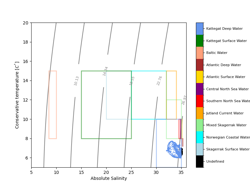
Create T-S Diagram for the transect#
We define here some temperature-salinity indexes based on the study of Danielssen et al. $1997^1$
1. Danielssen et al. (1997) - Oceanographic variability in the Skagerrak and Northern Kattegat, May–June, 1990
# --------------------------------------------------
# Water mass definitions
# --------------------------------------------------

water_masses = {
    "SSW": {"S": (20, 32), "T": (10, 15)},
    "NCW": {"S": (25, 32), "T": (10, 15)},
    "MSW": {"S": (32, 35), "T": (8, 12)},

    "JCW": {"S": (32, 34), "T": (10, 15)},
    "SNSW": {"S": (34.5, 34.8), "T": (8, 10)},
    "CNSW": {"S": (34.8, 35.0), "T": (8, 10)},

    "AW_upper": {"S": (35.00, 35.15), "T": (8, 10)},
    "AW_deep": {"S": (35.15, 35.32), "T": (7.2, 8)},

    "BW": {"S": (8.5, 10), "T": (8, 15)},
    "KSW": {"S": (15, 25), "T": (8, 15)},
    "KDW": {"S": (30, 35), "T": (5, 10)},
}

# --------------------------------------------------
# Colors
# --------------------------------------------------

color_map = {
    "Unknown": "black",
    "SSW": "lightblue",
    "NCW": "cyan",
    "MSW": "lightgreen",
    "JCW": "orange",
    "SNSW": "red",
    "CNSW": "purple",
    "AW_upper": "gold",
    "AW_deep": "brown",
    "BW": "lightsalmon",
    "KSW": "green",
    "KDW": "cornflowerblue",
}

wm_names = {
    "Unknown": "Undefined",
    "SSW": "Skagerrak Surface Water",
    "NCW": "Norwegian Coastal Water",
    "MSW": "Mixed Skagerrak Water",
    "JCW": "Jutland Current Water",
    "SNSW": "Southern North Sea Water",
    "CNSW": "Central North Sea Water",
    "AW_upper": "Atlantic Surface Water",
    "AW_deep": "Atlantic Deep Water",
    "BW": "Baltic Water",
    "KSW": "Kattegat Surface Water",
    "KDW": "Kattegat Deep Water",
}

# --------------------------------------------------
# Convert data to 1D arrays
# --------------------------------------------------

SA1 = np.asarray(SA).ravel()
CT1 = np.asarray(CT).ravel()
DEPTH = np.asarray(ds.z_rho.values).ravel()


# --------------------------------------------------
# Prepare classification arrays
# --------------------------------------------------

class_names = list(color_map.keys())
watermass_names = [wm_names[i] for i in color_map.keys()]
class_to_int = {name: i for i, name in enumerate(class_names)}
point_class = np.zeros(len(SA1), dtype=int)  # default = Unknown

# --------------------------------------------------
# Classify points
# --------------------------------------------------

for name, wm in water_masses.items():

    smin, smax = wm["S"]
    tmin, tmax = wm["T"]

    mask = (
        (point_class == 0) &
        (SA1 >= smin) & (SA1 <= smax) &
        (CT1 >= tmin) & (CT1 <= tmax)
    )

    point_class[mask] = class_to_int[name]

# --------------------------------------------------
# Define T-S grid
# --------------------------------------------------
Te = np.arange(0, 40, 1)
Se = np.arange(0, 40, 1)
Tg, Sg = np.meshgrid(Te, Se)
sigma_theta = gsw.sigma0(Sg, Tg)
cnt = np.linspace(sigma_theta.min(), sigma_theta.max(), 10)

# --------------------------------------------------
# Colormap setup
# --------------------------------------------------

colors = [color_map[name] for name in class_names]

cmap = ListedColormap(colors)

norm = BoundaryNorm(
    np.arange(len(class_names) + 1) - 0.5,
    cmap.N
)

# --------------------------------------------------
# Plot
# --------------------------------------------------

fig, ax = plt.subplots(figsize=(8, 6))

sc = ax.scatter(
    SA1,
    CT1,
    s=1,
    c=point_class,
    cmap=cmap,
    norm=norm,
    alpha=0.8,
    zorder=100
)


cs = ax.contour(
    Sg,
    Tg,
    sigma_theta,
    colors='grey',
    levels=cnt,
    zorder=1
)


for name, wm in water_masses.items():
    smin, smax = wm["S"]
    tmin, tmax = wm["T"]

    # draw box
    rect = patches.Rectangle(
        (smin, tmin),
        smax - smin,
        tmax - tmin,
        facecolor='None',
        edgecolor=color_map[name],
        alpha=0.5,
        linewidth=2
    )
    ax.add_patch(rect)

    # Compute center of box
    sc = (smin + smax) / 2


ax.clabel(cs, inline=True, fontsize=8)

ax.set_ylim(5, 20)
ax.set_xlim(5, 36)
ax.set_xlabel("Absolute Salinity")
ax.set_ylabel(r'Conservative temperature $[C^{\degree}]$')


# --------------------------------------------------
# Colorbar with class names
# --------------------------------------------------

cbar = plt.colorbar(
    ScalarMappable(cmap=cmap, norm=norm),
    ax=ax,
    ticks=np.arange(len(class_names))
)

cbar.ax.set_yticklabels(watermass_names, size=8)
fig.tight_layout
plt.show()

fig.tight_layout
plt.show()
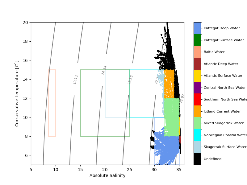
As a final example, we will create a T-S diagram for a long time series (whole 2025) extracted from one single grid point over time

ds = xr.open_dataset('./datasets/timeseries_norkyst_2025_deep.nc', engine='netcdf4')

# ---------------------------------------- #
# --- Conversion from S-coord to depth --- #
# ---------------------------------------- #
Zo_rho = (ds.hc * ds.s_rho + ds.Cs_r * ds.h) / (ds.hc + ds.h)
z_rho = ds.zeta + (ds.zeta + ds.h) * Zo_rho

ds.coords["z_rho"] = z_rho.transpose('ocean_time', 's_rho')

# ----------------- #
# --- CT, SA, p --- #
# ----------------- #

salt = ds.salt
temp_model = ds.temp

# Convert salinity and temperature from ROMS to TEOS-10 standards
p = gsw.conversions.p_from_z(ds.z_rho.values, 60.0) # Lat
SA = gsw.conversions.SA_from_SP(salt, p, 0.0, 60.0) # Lon, Lat
CT = gsw.conversions.CT_from_pt(SA, temp_model)
rho0 = gsw.pot_rho_t_exact(SA, CT, p, 0) # Ref level

# --------------------------------------------------
# Convert data to 1D arrays
# --------------------------------------------------

SA1 = np.asarray(SA).ravel()
CT1 = np.asarray(CT).ravel()

# --------------------------------------------------
# Prepare classification arrays
# --------------------------------------------------

class_names = list(color_map.keys())
watermass_names = [wm_names[i] for i in color_map.keys()]
class_to_int = {name: i for i, name in enumerate(class_names)}
point_class = np.zeros(len(SA1), dtype=int)  # default = Unknown

# --------------------------------------------------
# Classify points
# --------------------------------------------------

for name, wm in water_masses.items():

    smin, smax = wm["S"]
    tmin, tmax = wm["T"]

    mask = (
        (point_class == 0) &
        (SA1 >= smin) & (SA1 <= smax) &
        (CT1 >= tmin) & (CT1 <= tmax)
    )

    point_class[mask] = class_to_int[name]

# --------------------------------------------------
# Define T-S grid
# --------------------------------------------------
Te = np.arange(0, 40, 1)
Se = np.arange(0, 40, 1)
Tg, Sg = np.meshgrid(Te, Se)
sigma_theta = gsw.sigma0(Sg, Tg)
cnt = np.linspace(sigma_theta.min(), sigma_theta.max(), 10)

# ------------------- #
# --- Make figure --- #
# ------------------- #

fig, ax = plt.subplots(figsize=(8, 6))

sc = ax.scatter(
    SA1,
    CT1,
    s=1,
    c=point_class,
    cmap=cmap,
    norm=norm,
    alpha=0.8,
    zorder=100
)

cs = ax.contour(
    Sg,
    Tg,
    sigma_theta,
    colors='grey',
    levels=cnt,
    zorder=1
)


for name, wm in water_masses.items():
    smin, smax = wm["S"]
    tmin, tmax = wm["T"]

    # draw box
    rect = patches.Rectangle(
        (smin, tmin),
        smax - smin,
        tmax - tmin,
        facecolor='None',
        edgecolor=color_map[name],
        alpha=0.4,
        linewidth=2
    )
    ax.add_patch(rect)

    # Compute center of box
    sc = (smin + smax) / 2

ax.clabel(cs, inline=True, fontsize=8)

ax.set_ylim(5, 20)
ax.set_xlim(5, 36)
ax.set_xlabel("Absolute Salinity")
ax.set_ylabel(r'Conservative temperature $[C^{\degree}]$')

# --------------------------------------------------
# Colorbar with class names
# --------------------------------------------------

cbar = plt.colorbar(
    ScalarMappable(cmap=cmap, norm=norm),
    ax=ax,
    ticks=np.arange(len(class_names))
)

cbar.ax.set_yticklabels(watermass_names, size=8)
fig.tight_layout
<bound method Figure.tight_layout of <Figure size 800x600 with 2 Axes>>
Total running time of the script: (0 minutes 3.484 seconds)